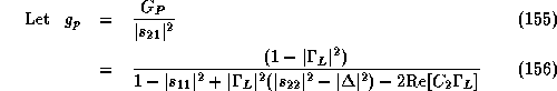
(156) can be rearranged as an equation of circle on

Recall operating power gain equation
![]()
(156) can be rearranged as an equation of circle on ![]() plane
plane
For each value of ![]() , we have a corresponding
, we have a corresponding ![]() circle with
circle with
![]()
![]()
Note that the centers of ![]() circles are always on the line drawn between
circles are always on the line drawn between ![]() and the origin of the
and the origin of the
![]() plane. The radius of
plane. The radius of ![]() circle is getting smaller for a larger
circle is getting smaller for a larger ![]() .
In case of an unconditionally stable device, when
.
In case of an unconditionally stable device, when ![]() ,
, ![]() reaches its maximum.
reaches its maximum.
![]()
so as ![]()
![]()
In case of a potentially unstable device, when ![]() , i.e.,
, i.e., ![]() , the
, the ![]() circle equals to input stability circle.
circle equals to input stability circle.
![]()
![]()
Example In a 50 ![]() system, a transistor has the following S-parameter at 1.3 GHz.
Plot a few constant operating power gain circles.
system, a transistor has the following S-parameter at 1.3 GHz.
Plot a few constant operating power gain circles.
![]()
![]()
Solution ![]() dB.
dB.
![]()
At maximum operating power gain, the constant gain circle becomes a point
with ![]() , and the load reflection coefficient is
, and the load reflection coefficient is
![]()
We can calculate the corresponding input reflection coefficient for this load.
![]()
Hence, if the source is conjugately matched with the amplifier, then the source reflection
coefficient becomes
![]()
Note that the results are the same as the optimum terminations ![]() ,
,![]() .
.
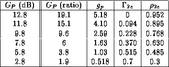
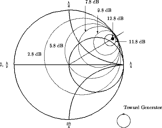
Figure 19: A set of constant operating gain circles plotted on a Smith chart